
Welcome to the Wheelhouse, a series of blogs from Ebiquity’s Marketing Effectiveness team.
The “Bayesian versus traditionalist” tribal conflict has reached the media mix industry. Until recently, this had been a rarefied debate, limited to the data scientists who work in our marketing effectiveness practice. But there’s evidence that is shifting from the theoretical to the practical in the sector.
The debate itself is not new news in academic circles. What has changed recently is that we are seeing Bayesian methods cropping up in pitches, in client briefs, and as a selling point for competitor platforms. Even Google has published “Lightweight MMM” – a Bayesian code package – and this has only served to bolster the credibility of the approach.
Bayesian statistics is a huge field and a genuinely different way of thinking that is slightly out of my personal comfort zone. I wrote this article as a short primer, to clarify in my own mind how Bayesian methods apply to ROI measurement and MMM. If you’ve started to hear more about Bayesian MMM and are keen to find out more, read on. And do be prepared for a few charts.
The starting point
Compared to traditional, ordinary, least-squares (OLS) econometrics, Bayesian modelling requires a more probabilistic mindset right from the start. First off, you define an expected outcome along with a reasonable range to reflect your level of certainty. This input can be based on your domain knowledge or other data. This is called a prior.
Then, your model will evaluate the evidence. Unlike an OLS model – a model that returns a single best estimate for each factor under analysis – Bayesian regression runs millions of simulations and returns a probability that a specific set of outcomes is possible, given the data. Under certain narrow assumptions, the central estimate is identical to old-school approaches like ordinary least squares (OLS) or, indeed, the frequentist maximum likelihood estimation (MLE).
Finally, the model will calculate a so-called posterior. This is the final answer on your ‘exam paper’. It combines the information in your prior with the evidence from the data to give an updated final estimate. As before, it is not a single number, but a distribution of possible values and their associated likelihood. Let’s look at how this works in the more familiar territory of media ROI measurement.
A worked example
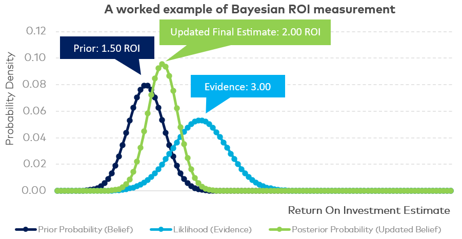
- We believe that the ROI on a media line is 1.50 – that is, for every £1 invested, we expect to generate returns of £1.50. And there’s about an 80% chance that the ROI falls between 0.90 and 2.10. This is our prior.
- The evidence in the data suggests that the ROI is most likely to be around 3.00. There is about an 80% chance it falls between 2.00 and 4.00. This distribution suggests a slightly higher level of uncertainty than allowed for in our prior.
- Both curves are combined to arrive at the final estimate. The ROI is expected to be 2.00. But we don’t just care about the central estimate, we have a range such that we can see there is an 80% chance the number falls between 1.50 and 2.50. This is our posterior.
Now, at this point it is worth saying that the Bayesian approach is not as arbitrary as it sounds. If the sample size is good and you do not have collinearity – that is, correlation between the predictor variables in the model – then the quality of the evidence will outweigh the prior and have more sway in the final number. This is illustrated in the example below.

What is the selling point of Bayesian regression in MMM?
There are four main arguments made for the use of Bayesian regression in marketing mix modelling.
- Bayesian regression allows granular reporting because it deals well with collinearity.
- Bayesian regression deals well with lower media budgets.
- Bayesian regression copes well with smaller sample sizes, typical in MMM
- Bayesian regression allows faster updates.
Let’s talk about collinearity first. Collinearity means your explanatory variables are correlated, which is kryptonite to econometric models. Unfortunately, this is also very common. Media planners love bursts and synergies, so in practice you see this issue come up often.
There are formal tests for collinearity in a traditional econometric model, but the usual giveaway is that your ROI estimates bounce around wildly as you tweak the model.
In a Bayesian model with collinearity you don’t get an unstable single best estimate, instead you get a hopelessly broad likelihood curve. This is the model’s equivalent of looking at the problem and shrugging its shoulders.
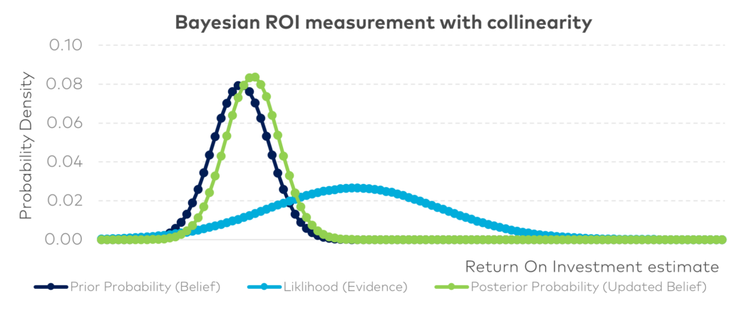
In the example shown above, the data suggests that the ROI is 3.00, with 80% probability that it falls between 1.00 and 5.00. The prior is 1.50 and the updated posterior view is 1.70. So in this case, it is the analyst rather than the data has done most of the work to determine the outcome.
This principle is also how Bayesian models can be used to manage smaller budget media lines, which are typically volatile in MMM models. The Bayesian framework allows the analyst to influence the estimate back to common sense levels.
Reappraising Bayesian models
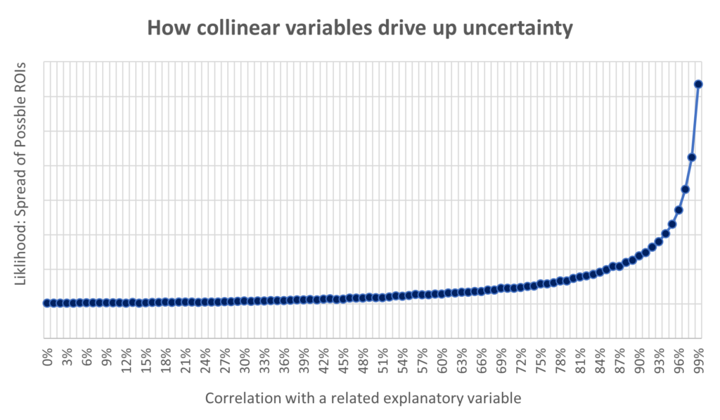
In Richard McElreath’s excellent book Statistical Rethinking he runs a simulation to show how two correlated factors combine to increase uncertainty. In this simulation around the 90% correlation mark, the measurement uncertainty simply explodes along with the range of possible outcomes. In the MMM sector, we see this pattern all the time for closely-related channels like TV and VOD. Correlation is often 90%-95%. This is because VOD budgets are set as a share of TV budgets.
Bayesian models offer a tidy solution in that they allow you to lean on your priors to create more stability. They can also be set up to solve a joint estimate on multiple media lines at the same time, with a prior expectation about how much those components can vary – in a hierarchical model or multilevel setup. What they can’t do is get rid of the identification problem on a fundamental level. The problem is still there, there is no new information, and it is simply being managed.
This bring us to the fourth major selling point: faster turnaround times.
Compared with traditional MMM, Bayesian models run relatively slowly. The way they improve turnaround times is that you can add new data to a model with priors based on the results that have been previously communicated to the client. This has a stabilising effect, as updated results are basically weighted towards previous results, especially if you choose to set relatively tight priors. With a more stable model you can save time grappling with data inconsistencies so you can publish results sooner.
Bayesian models in the boardroom
That’s the technical detail – explained, I believe, as simply as possible, and illustrated with straightforward theoretical charts. Let’s put the technical argument on one side and consider how this plays out in the boardroom, an environment with no time or place for the niceties of different schools of statistical modelling.
More granularity and faster turnaround times are obviously good things – just the kind of outcomes CFOs are always asking for. And yet it’s very hard to deny that, if CFOs genuinely understood how Bayesian MMM works, they wouldn’t be thrilled about it. They would be well within their rights to ask pointy questions about whether the CMOs’ budget request oughtn’t to come with caveats and health-warmings.
In the true Bayesian spirit, it would be better to present the prior and posterior distribution to decision makers rather than a single number, but this kind of hand waving will get your predictions thrown out of the window because they just don’t provide enough certainty. In practice, CMOs go to the boardroom with best estimates and try to keep their story simple.
The Bayesian approach makes it too easy to avoid difficult conversations. If you add new data to a model and discover that you need to downgrade your previous ROI estimate, the right thing to do would be to talk through the implications of that change. Or you could lean on the prior to ensure a more consistent narrative. If your client asks whether you can split a media line into a dozen sub-channels, the right thing to do is advise against this. But with a Bayesian model, it’s just too tempting to let it slide rather than challenge the brief.
A Groucho Marx development plan?
So, mixed feelings. Bayesian ROI measurement is technically neat; it feels like an aspirin to an MMM induced headache. The main danger of Bayesian MMM is that it entrenches some bad habits that are already common in our sector: not speaking openly to clients about the limits of analytics, overpromising in a pitch setting, over-fitting models, and artificially enforcing consistency of model outputs. And that’s just for starters.
Despite these understandable misgivings, Ebiquity is investing in building Bayesian tools. Reading this blog, you might think of the Groucho Marx line: “Those are my principles, and if you don’t like them … well, I have others.” We have nothing against Bayesian methods. They are just another tool, and they can be used and abused just like any other statistical method.
We are adding Bayesian regression to our modelling platform alongside OLS, elastic net, dynamic linear regression, and genetic algorithms. We give our consultants as much choice as possible to pick the best tools for the job to answer the client brief. What matters is the investment advice, and at the end of the day, the regression method used is just a footnote.
Group Director Nic Pietersma considers the impact and importance of a long-running debate and difference of approach in academic statistics on marketing science in the second edition of the Wheelhouse, marketing effectiveness blog.
Feel free to get in touch with the Ebiquity team to further discuss these important updates and take proactive steps to reduce wasteful practices. Reach out now.